BAMBA Kafoumba
Email: bambakaf.sfa@univ-na.ci
© 2019 Sift Desk Journals. All Rights Reserved
VOLUME: 4 ISSUE: 3
Page No: 403-414
BAMBA Kafoumba
Email: bambakaf.sfa@univ-na.ci
MASSAPIHANHORO Ouattara Pierre, BAMBA Kafoumba*, KONE Mamadou Guy-Richard, EHOUMAN Ahissan Donatien, N’GUESSAN Nobel Kouakou, ZIAO Nahossé
Laboratoire de Thermodynamique et Physico-Chimie du Milieu, Université Nangui Abrogoua
BAMBA Kafoumba, Predictive study of the Bioconcentration of Organochlorine Compounds by a QSPR Model(2020)Journal of Computational Chemistry & Molecular Modeling 4(3) pp:403-414
Despite their effectiveness, most organochlorine pesticides are banned. Indeed, these compounds are considered very persistent. To understand this persistence, we carried out a modeling study of the bioconcentration factor. This study permitted to understand that bioconcentration factor is well described by hydrogen percentage (%H), constant volume heat capacity (Cv), partition coefficient (Log P) and density (D).These descriptors constituted the explicative and predictive parameters of the bioconcentration of organochlorine compounds. This study was performed by analyzing the correlation matrix, of a multiple linear regression (MLR) model, the contribution of the descriptors and the applicability domain of the descriptors. The model obtained displayed good statistical indicators according to the principles established by the Organization for Economic Cooperation and Development (OECD). MLR statistical indicators reveal more effective predictions with coefficient of determination R2 = 0.983, coefficient of determination adjusted R2ajusted = 0.979, standard error S=0.179, cross-validation correlation coefficient R2cv = 0.983 and Fisher's test F= 221.206. This model is acceptable with R2-R2cv= 0,0003. The results obtained suggest that combining these descriptors could be useful for predicting the property of bioconcentration. In addition, the percentage of hydrogen (% H) is the priority descriptor for the prediction of this bioconcentration for news organochlorine pesticides.
Keywords: toxicity, quantum descriptors, physicochemical descriptors, cook distance
Organochlorine Pesticides (OCP) are organic compounds obtained by the chlorination of various unsaturated hydrocarbons. Indeed, it is admitted that the molecules with more than 4 chlorine atoms are resistant to degradation and are considered as long-lasting compounds in the marine environment[1]. They are assumed to bioaccumulate in fatty tissues and to potentially damage the marine resources [2].The fate of environmental pollutants is a fundamental aspect of ecotoxicology that makes therefore the understanding of the bioaccumulation’s process a necessity.
It is well known that organochlorine pesticides are concentrated in biological systems and precisely in adipose tissue. Actually, they bioaccumulate throughout the food chain, reaching higher concentrations in higher animals such as humans[1] that triggers the phenomenon of the biomagnification. Thus, Bodin[3] highlighted the bioaccumulation of the most persistent polychlorobiphenyl congeners along the spider crab food chain. In the same study, she showed that bioaccumulation was influenced by organotropism, diet and age.
Organotropism refers to the process by which certain molecules are directed and possibly permanently stored by certain organs, preferably or even almost exclusively. Besides, diet is the sum of food consumed by a person or other organism.
Traore et al.[4] studied the bioaccumulation of organochlorine pesticides in cow's milk and butter traditionally produced in certain regions of Côte d'Ivoire. Even though the residue levels found are below the tolerable thresholds set by international standards, the authors nevertheless draw the attention of consumers to the dangers that could result from the phenomenon of bioaccumulation. The curdled milk and eggs consumed in Côte d'Ivoire are not entirely safe from contamination by organochlorine pesticides [5]. It was shown for instance that the fish of the Lake of Buyo in Côte d'ivoire is also contaminated by the organochlorine pesticides [6]. Besides, Benbakhta et al.[7] showed that some aquatic species in the Moulay Bousselham lagoon in Morocco are contaminated with organochlorine pesticides.
In 2016, Yohannes et al.[8] studied the contamination of four species of bird. This study revealed that the maximum of 1-chloro-4-[2,2-dichloro-1-(4-chlorophenyl)ethenyl]benzene (p,p'-DDE) concentrations might have been enough to cause egg shell thinning, and have an impact on survival and breeding success of the bird species in the Rift Valley region. The rate of detection of 1-chloro-4-[2,2,2-trichloro-1-(4-chlorophenyl)ethyl]benzene (p, p' – DDT) permitted the authors to suggest a release of fresh DDT into the environment.
Previously in the years 1970 certain authors [9-12] revealed that the bioaccumulation of the organochlorinated compounds is related to their high lipo-solubility and their weak hydro-solubility. But different terms are used to describe the processes that define the fate of contaminants in different compartments of the environment (bioaccumulation, bioconcentration and Biomagnification). It is thus necessary to define these terms.
According to the report of the French Research Institute for the Exploitation of the Sea [9], bioconcentration in an organism is the accumulation of a chemical substance only via water, breathing or direct contact with the skin.
Biomagnification involves an increase of concentration in organisms at the upper trophic level. The bioaccumulation or the bioconcentration or the biomagnification of a molecule in an organism is related to the physicochemical properties of this molecule. The bioconcentration factor (BCF) is then defined as the equilibrium ratio between the contaminant concentration in the body (CB ) on the dissolved contaminant concentration in water (CED ):

When the bioconcentration factor is high, the chemical compound has a high capacity to store in the biological environment studied. This factor therefore makes it possible to evaluate the capacity of degradation or accumulation of a chemical compound in the environment.
The bioaccumulation of a molecule is related to its physico-chemical properties. If persistence is often considered as a result of the long half-life of the pollutant or its continued release into the marine environment, it may also be the result of its bioaccumulation.
The main objective of this study is to perform a QSPR study of organochlorine compounds to determine the descriptors that influence their bioconcentration factor.
2.1. Materials
2.1.1. Selection of Data Set
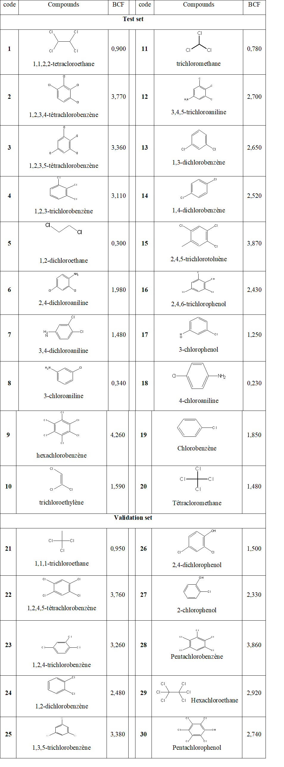
We investigated about 30 molecules where 20 were used for the test set and 10 for the validation set. Their values for the bioconcentration factor of organochlorine molecules for fish are well known and displayed in Table 1 [14].
Table 1 : Data Set
2.1.2. Methods of Calculation
We used Gaussian 03 software[15] to optimize each molecule into DFT method with Becke‘s three-parameter hybrid method and the Lee-Yang-Parr B3LYP functional [16]employing 6-311++g(d,p) basis set. The split-valence and triple-dzeta bases (6-311 ++ g (d, p)), being sufficiently extensive and taking into account the polarization functions are important for taking into account the free doublets of the heteroatoms. The use of this method was justified by the way that DFT methods present the best compromise among calculation time and quality, since the electronic correlation is taken into account and functional calculus and B3LYP seems adapted well for the study of the organic compounds [17].
2.1.3. Molecular Descriptors
Four descriptors were calculated. These descriptors are composed of one quantum descriptor and three physico-chemical descriptors. The combination of descriptors belonging to different categories (constitutional, topological, quantum-chemical…) led to improve QSPR performances[18]. This improvement was shown in our first article [19].These descriptors include:
Density (D): density is a steric parameter. It is calculated by ACD Lab Chem Sketch Software. This parameter is related with the bulk and size of the substituents [20]

Partition coefficient (Log P): Partition coefficient allows to measure the differential solubility of a neutral substance between the immiscible liquids and thereby, a descriptor of hydrophobicity (or the lipophilicity) of a neutral substance. LogP is usually used in its logarithmic form(log P)[20,21]. Indeed, if logP is positive and very high, this expresses that the molecule considered is more soluble in octanol than in water, which reflects its lipophilic character and if the log P is negative this means that the molecule considered is hydrophilic. A null value of LogP means that the molecule is as soluble in both middles. In this work, the Chemsketch software [22] allowed us to determine the values of the LogP. In practice, lipophilicity is expressed by the decimal logarithm of the logP partition coefficient. So :
Constant volume heat capacity (Cv) : the constant volume heat capacity of a compound is a size making it possible to quantify the possibility that has a compound to absorb or restore energy by heat exchange during a transformation during which its temperature varies. It is the energy which it is necessary to bring to a compound to increase its temperature of one Kelvin. It is an extensive size, i.e. increases with the quantity of the matter.
Percentage of hydrogen (%H) : the percentage of hydrogen atom is a quantity which makes it possible to quantify the proportion occupied by the hydrogen atoms on the set of atoms that compose the molecule. A high value of this quantity shows that the molecule contains more hydrogen atoms.
2.2. Methods
2.2.1. Descriptive Analysis
The partial correlation coefficient calculation was performed using a principal component analysis that is implemented in the XLSTAT [23] software.
2.2.2. Statistical Analysis
The choice of the best model satisfies the criteria of statistical analysis which are:
It measures the share of the experimental variance explained by the model compared to the total variance. Its value is between 0 and 1. The closer the value of R² is to 1, the more the theoretical and experimental values are well correlated. Furthermore, a weak value of means that the model has a weak explicative power and descriptors have no effect on the property explained.

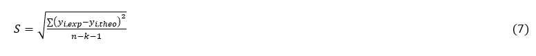
where:
yi,exp : The experimental value of antifungal activity
yi,theo : The theoretical value of the activity
y̅i,exp : The mean value (average) of the experimental values of activity.
High value of the adjusted coefficient of determination(R2adjusted≥0.6)
It allows to measure the robustness of a model unlike . It is used in multiple linear regression because it takes into account the number of descriptors of the model.

Where :
n: the sample size and
k: the number of independent variables in the regression equation.
High value of the Fischer coefficient (F).
This coefficient allows to test the overall significance of the linear regression [25].

Where : n is the sample size and is the number of independent variables in the regression equation
High value of the cross-validation coefficient (R2CV>0.5)[24]. It measures the accuracy of the prediction on the test set.

Low values of the standard deviation (S): Standard deviation is an indicator of dispersion. It provides information on how the distribution of data is done around the average. when its value is proximate to 0 the fit is good, and we have the higher reliability of the prediction. A standard deviation greater than 0.50 indicates a large dispersion of the data around the mean.
We used Multiple Linear Regression (MLR) method of XLSTAT to establish QSPR model.
The statistical technique of multiple linear regression (MLR) is used to study the relationship between a dependent variable (Property) and several independent variables (descriptors). This statistical method minimizes the differences between the experimental value and predicted values. It is the most common tool for studying multidimensional data. It is based on the following pre-programmed XLSTAT functions:

Where a, b, c, d, represent the parameters and x1, x2, x3, x4, represent the variables.
2.2.3. Acceptance Criteria for a QSPR Model
According Eriksson et al. [26 ] and N’Dri et al [27],the performance of a mathematical model is proved by a value of for a satisfactory model when R2cv> 0.9 the model is described as excellent. According to them, for a test set, a model will be accepted if the condition R2- R2cv< 0.3 is respected.
The set of descriptor values for the twenty (20) organochlorine compounds in the test set and the ten (10) other molecules in the validation set are presented in Table 2.
Table 2: Physico-chemical and quantum descriptors and the bioconcentration factor (BCF) of the test and validation sets
|
Cv(Cal/Mol-Kelvin ) |
%H |
D |
LogP |
BCF |
|
|
Test set |
|||||
|
1 |
22.213 |
1.2 |
1.556 |
2.17 |
0.900 |
|
2 |
32.291 |
0.93 |
1.573 |
4.18 |
3.770 |
|
3 |
32.42 |
0.93 |
1.573 |
4.31 |
3.360 |
|
4 |
28.573 |
1.67 |
1.448 |
3.77 |
3.110 |
|
5 |
15.167 |
4.07 |
1.173 |
1.41 |
0.300 |
|
6 |
30.936 |
3.11 |
1.401 |
2.74 |
1.980 |
|
7 |
28.682 |
3.11 |
1.401 |
2.51 |
1.480 |
|
8 |
24.919 |
4.74 |
1.23 |
1.81 |
0.340 |
|
9 |
39.984 |
0 |
1.767 |
4.89 |
4.260 |
|
10 |
17.123 |
0.77 |
1.474 |
2.26 |
1.590 |
|
11 |
13.8 |
0.84 |
1.5 |
1.76 |
0.780 |
|
12 |
34.875 |
2.05 |
1.54 |
3.27 |
2.700 |
|
13 |
24.899 |
2.74 |
1.297 |
3.42 |
2.650 |
|
14 |
24.877 |
2.74 |
1.297 |
3.34 |
2.520 |
|
15 |
34.655 |
2.58 |
1.38 |
4.28 |
3.870 |
|
16 |
31.754 |
1.53 |
1.595 |
3.58 |
2.430 |
|
17 |
25.926 |
3.92 |
1.287 |
2.4 |
1.250 |
|
18 |
27.211 |
4.74 |
1.23 |
1.76 |
0.230 |
|
19 |
21.058 |
4.48 |
1.11 |
2.81 |
1.850 |
|
20 |
18.19 |
0 |
1.697 |
2.86 |
1.480 |
|
Validation set |
|||||
|
21 |
19.988 |
2.27 |
1.393 |
2.1 |
0.950 |
|
22 |
32.364 |
0.93 |
1.573 |
4.23 |
3.760 |
|
23 |
28.634 |
1.67 |
1.448 |
3.82 |
3.260 |
|
24 |
24.794 |
2.74 |
1.297 |
3.28 |
2.480 |
|
25 |
28.749 |
1.67 |
1.448 |
4.04 |
3.380 |
|
26 |
29.475 |
2.47 |
1.458 |
2.99 |
1.500 |
|
27 |
25.785 |
3.92 |
1.287 |
2.04 |
2.330 |
|
28 |
40.718 |
0.38 |
1.804 |
4.78 |
3.860 |
|
29 |
30.772 |
0 |
1.821 |
4.47 |
2.920 |
|
30 |
40.718 |
0.38 |
1.804 |
4.78 |
2.740 |
3.1. Matrix of Correlation
The matrix of correlation is made out with Principal component analysis. This matrix shows that no interdependence exists between molecular descriptors used because partials correlation coefficients between descriptors are less than 0.95 (ri<0.95)[26,28-34].The following correlation matrix displayed in Table 3 is obtained.
Table 3 : Matrice de corrélation (Pearson (n))
|
Variables |
BCF |
Cv |
%H |
D |
LogP |
|
BCF |
1 |
||||
|
Cv |
0.726 |
1 |
|||
|
%H |
-0.542 |
-0.320 |
1 |
||
|
D |
0.512 |
0.552 |
-0.916 |
1 |
|
|
LogP |
0.923 |
0.804 |
-0.635 |
0.668 |
1 |
We used these descriptors to establish the QSPR model.
3.2. Equation of Model
The equation of the QSAR model with the statistical data is presented below. This model obtained gives the relation between the bioconcentration factor (BCF) and the theoretical descriptors of organochlorine compounds. The negative or positive value of the coefficient of a descriptor in the model translates the effect of proportionality between the evolution of the property and this parameter of the regression equation. The negative value indicates that when the value of the descriptor is high, the property decreases. The positive sign indicates the opposite effect.

N=20, R2=0.9833 , R2ajusted= 0.979, S =0.179 , F= 221.206 Pvalue< 0.0001, a=0.005,
R2CV= 0.9830,
The negative correlation coefficient between the percentage of hydrogen (% H) and the density (d) indicate that these two variables are inversely proportional, i.e. the increase of the percentage of hydrogen (% H) or the density causes the reduction of the bioconcentration factor (BCF) in the model.
The greatest values of R2= 0.983 ; R2ajusted= 0.979 and the lowest values of S=0.179 and Pvalue< 0.0001 shows the strong relation which exists between the bioconcentration factor and the selected descriptors. This model is very highly significant (high value of Fischer parameter: F = 221.206).Then both R2CV= 0.979 > 0.9 and prove that this model is excellent.
Analysis of QSPR model equation reveals that the bioconcentration increases when and increase then and decrease. Considering that lipophilia increases with the number of chlorine atom, we can say that the factor of bioaccumulation increases when the number of chlorine atom increases.
The regression line between the experimental and theoretical BCF of the test and the validation set is illustrated in Figure 1. The value of the determination coefficient R2= 0.983 and the low value of the mean square error S=0.179 prove a good similarity between the predicted and experimental values. This good similarity is also shown in Figure 2.
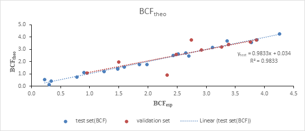
Figure 1: Regression line of the test and validation set
The different points of the test set are all close to the regression line. This proximity attests a good correlation between the experimental values and those predicted. This regression line indicates that:

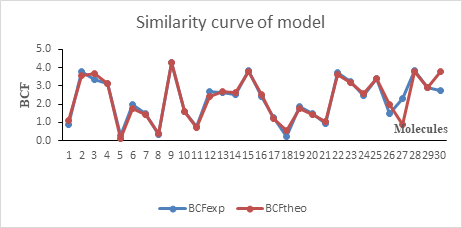
Figure 2: Similarity curve of the experimental and predicted values model
Figure 2 shows that both predicted and experimental values and almost the same. They also evolve in the same directions. However, both the molecules 27 and 30 that belong to the validation set display different values.
Furthermore, the low standard error value (S) which is 0.179 for this model attests a good similarity between the predicted and experimental values.
3.3. Contribution of Descriptors
The contributions of the molecular descriptors in the prediction of the organochlorine molecules bioconcentration factor are illustrated by the Figure 3. The classification of the contribution of the descriptors in the model is as follows:
%H(-0.874)>D(-0.812)>LogP(0.640)>Cv (0.430)
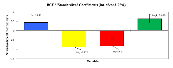
Figure 3: Contribution of descriptors
According to the contribution of these descriptors, the percentage of hydrogen (% H) displays the highest normalized coefficient (-0.874) followed by the density (D) with -0.812. The constant volume heat capacity (Cv) has the lowest coefficient (0.430) compared to other descriptors. It should be noted that the percentage of hydrogen (% H) is the most influential physico-chemical descriptor. Thus, to improve the bioconcentration factor in the synthesis of new organochlorine pesticides, it is necessary to speculate more on the percentage of hydrogen (% H).
Furthermore, we will use the cook distance (di) [35] to determine the applicability domain. This notion is another measure of the impact of the respective observation on the regression equation. It represents the difference between the calculated coefficients and the values that would have been obtained if the corresponding observation had been excluded from the analysis. To evaluate the influence of a point i on the regression, it is removed from the calculation of the coefficients. Then, we compare the predictions with the complete model constructed with all the points and the model constructed without the point i. If the difference is high, then, the point is assumed to play an important role in the estimation of the coefficients. We define subsequently the threshold value from which we can say that the influence is exaggerated. The simplest rule is: . But it is considered a little too permissive, wrongly letting doubtful points escape; we sometimes prefer the following more demanding provision [36,37]:
di>4/(N-k-1)
With k standing for number of predictors and N the number of compounds.
All distances must be of the same order of magnitude; if not, there is good reason to believe that the respective observation (s) bias the regression coefficient estimate. In our article, points with a great Cook distance
di>4/(N-k-1) i.e di>4⁄((20-4-1) )=0.2667] are considered to belong to the domain of applicability. The cook distances for our molecules have been given in the Table 4 and are visible in the Figure 4.a and in the Figure 4.b.
Table 4 : Cook’s distance of molecules
|
Compounds |
Cook’s distance |
|
1,1,2,2-tetracloroethane |
0.100 |
|
1,2,3,4-tétrachlorobenzène |
0.044 |
|
1,2,3,5-tétrachlorobenzène |
0.141 |
|
1,2,3-trichlorobenzène |
0.002 |
|
1,2-dichloroethane |
0.060 |
|
2,4-dichloroaniline |
0.053 |
|
3,4-dichloroaniline |
0.004 |
|
3-chloroaniline |
0.012 |
|
Hexachlorobenzène |
0.001 |
|
Trichloroethylène |
0.002 |
|
Trichloromethane |
0.014 |
|
3,4,5-trichloroaniline |
0.147 |
|
1,3-dichlorobenzène |
0.006 |
|
1,4-dichlorobenzène |
0.023 |
|
2,4,5-trichlorotoluène |
0.023 |
|
2,4,6-trichlorophenol |
0.012 |
|
3-chlorophenol |
0.002 |
|
4-chloroaniline |
0.316 |
|
Chlorobenzène |
0.037 |
|
Tétracloromethane |
0.272 |
|
1,1,1-trichloroethane |
0.015 |
|
1,2,4,5-tétrachlorobenzène |
0.022 |
|
1,2,4-trichlorobenzène |
0.004 |
|
1,2-dichlorobenzène |
0.015 |
|
1,3,5-trichlorobenzène |
0.000 |
|
2,4-dichlorophenol |
0.137 |
|
2-chlorophenol |
0.560 |
|
Pentachlorobenzène |
0.026 |
|
Hexachloroethane |
0.002 |
|
Pentachlorophenol |
1.367 |
The analysis of the cook distance shows that all the molecules used have Cook distances lower than the limit value (di =0.2667) except for 4 molecules. These compounds are 4-chloroaniline (di = 0,316), tétracloromethane (di = 0,272), 2-chlorophenol (di = 0,560), pentachlorophenol (di = 1,367). These compounds are considered as not belonging to the applicability domain.These erroneous predictions could probably be attributed to wrong experimental data or to the structural of theses outliers.
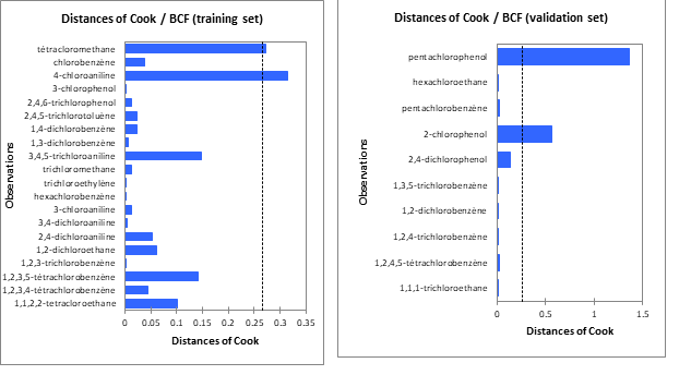
|
Figure 4.a : Cook’s distance of tests molecules |
Figure 4.b : Cook’s distance of validation molecules |
These different figures make it possible to visualize the four compounds whose is greater than the limit value (0.267).
Organochlorine compounds are compounds well known to be bio accumulative. The pesticides in this family are very effective. But because of their concentration in the environment, these pesticides have been banned from use. In order to give them a second chance, we have undertaken a series of studies in which it is located. In this study, our objective was to carry out a QSPR study in order to understand the phenomenon of bioconcentration. The parameters obtained R2 = 0.9833, R2ajusted =0.979, 0.179, F= 221.206, Pvalue< 0.0001, a=0.005, R2cv = 0.9830, R2- R2cv= 0.0003 show that the bioconcentration factor is well described by the constant vapor heat capacity ( , hydrogen percentage , density and lipophilicity . The QSPR equation obtained shows also that the factor of bioaccumulation increases when the number of chlorine atom increases. Because when the number of chlorine atoms decreases, the percentage of hydrogen atom increases and the lipophilicity decreases. The above equation can therefore be used to predict the bioconcentration factors of new organochlorine compounds. In perspective, we will determine the descriptors that influence the half-life time of organochlorine compounds and then propose less toxic, less bio-accumulative and less persistent organochlorine pesticides.
M.H. Debouge, J.P. Thome &CH. Jeuniaux, «Bioaccumulation de trois insecticides organochlorés (lindane, dieldrine, et DDT) et des PCB chez plusieurs espèces de forumis [hymenoptera-formicidae] en Belgique. »Entomophagavol. 32, pp. 551-561, (1987).
View ArticleStellio Casas, «Modélisation de la bioaccumulation des contaminants organiques (PCB,DDT et HAP) chez la moules Mytilusgalloprovincialis en milieu méditerranéen.», Rapport de recherche , RST/LER/PAC/07-14, Ifremer, p. 241, (2007).
Nathalie Bodin, « Contamination des crustacés décapodes par les composés organohalogénés. Etude détaillée de la bioaccumulation des PCB chez l'araignée de mer Maja brachydactyla.» Océan, Atmosphère. Université de Bretagne occidentale - Brest, p. 148 (2005).
Sory Karim TRAORE, Ardjouma DEMBELE, Koné MAMADOU Véronique MAMBO, Pierre LAFRANCE, Yves-Alain BEKRO et Pascal HOUENOU. «Contrôle des pesticides organochlorés dans le lait et produitslaitiers : Bioaccumulation et risques d'exposition.» Afrique SCIENCE vol. 04, pp. 87 - 98 (2008).
David Léonce KOUADIO, Serge Guy Ano EHOUMAN, Baba Donafologo SORO, Moussa DIARRA, Mohamadou Lamine DOUMBIA, Ladji MEITE, Koné MAMADOU, Ardjouma DEMBELE et Sory Karim TRAORE. «Contamination du lait caillé et de l'œuf consommé en Côte d'Ivoire par des pesticides organochlorés.» Afrique SCIENCE vol.10 pp. 61 - 69, (2014).
K. S. Traore, K. Mamadou, A. Dembele, « Contamination des peuplements de poissons du lac de BUYO. » J. Soc. Ouest-Afr. Chim., vol. 16, pp. 137-152, (2003).
Benbakhta Bouchaib, Fekhaoui Mohamed, El Abidi Abdellah, Idrissi Larbi, et Lecorre Pierre. « Résidus de pesticides organochlorés chez les bivalves et les poissons de la lagune de Moulay Bousselham (Maroc).» Afrique SCIENCE vol. 03, pp. 146 - 168, (2007).
Yared Beyene Yohannes , Yoshinori Ikenaka, Shouta M.M. Nakayama, Hazuki Mizukawa, Mayumi Ishizuka, «DDTs and other organochlorine pesticides in tissues of four bird species from the Rift Valley region» Ethiopia, Sci Total Environ, vol. 574, pp. 1389-1395, (2016). PMid:27539819
View Article PubMed/NCBIJohnson, B. Th., Saunders,C. R. & Sanders,H. O, «Biologicalmagnification and degradation of DDT and aldrin by freshwater invertebrates.»J. Fish. Res. Bd Can., vol. 28, pp. 705-9, (1971).
View ArticleUlmann, E. «Lindane, monographie d'un insecticide.», (Sehillinger, K., ed.), Verlag. Freiburg im Breisgau, pp. 383, (1972).
Hutzinger,O, Safe, S. & Zitko, V. «The chemistry of PCB's.»CRC Press Inc., Boca Raton, p.269, (1974).
Portmat, J.E. «Evaluation of the impact on the aquatic environment of HCB isomers, HCB, DDT ( + DDE and DDD), heptachlor ( + heptachlor epoxide) and chlordane.»CEE Environ., vol. 488, p. 337, (1979).
Gobas, Frank A.P.C. et al «Bioconcentration and Biomagnification in the Aquatic Environment » in Frank A.P.C. Gobas and Heather A. Morrison. Handbook of Property Estimation Methods for Chemicals. Environmental and Health Sciences. CRC Press LLC,pp. 210-252, (2000). PMid:10948288
View Article PubMed/NCBIVishnu Kumar Sahu and Rajesh Kumar Singh«Prediction of the Bioconcentration Factor of Organic Compounds in Fish»Clean, vol. 37, pp. 850-857,(2009), DOI: 10.1002/clen.200900170
View ArticleFrisch M. J., Trucks G. W., Schlegel H. B., Scuseria G. E., Robb M. A., Cheeseman J. R., Montgomery J. A., Jr., Vreven T., Kudin K. N., Burant J. C., Millam J. M., Iyengar S. S., Tomasi J., Barone V., Mennucci B., Cossi M., Scalmani G., Rega N., Petersson G. A., Nakatsuji H., Hada M., Ehara M., Toyota K., Fukuda R., Hasegawa J., Ishida M., Nakajima T., Honda Y., Kitao O., Nakai H., Klene M., Li X., Knox J. E., Hratchian H. P., Cross J. B., Adamo C., Jaramillo J., Gomperts R., Stratmann R. E., Yazyev O., Austin A. J., Cammi R., J. J., Zakrzewski V. G., Dapprich S., Daniels A. D., Strain M. C., Farkas O., Malick D. K., Rabuck A. D., Raghavachari K., Foresman J. B., Ortiz J. V., Cui Q., Baboul A. G., Clifford S., Cioslowski J., Stefanov B. B., Liu G., Liashenko A., Piskorz P., Komaromi I., Martin R. L., Fox D. J., Keith T., Al-Laham M. A., Peng C. Y., Nanayakkara A., Challacombe M., Gill P. M. W., Johnson B., Chen W., Wong M. W., Gonzalez C., and Pople J. A. Gaussian 03, Revision B.02. Gaussian, Inc.,
C. Lee, W. Yang, and R.G. Parr, « Development of the Colle-Salvetti correlation-energy for into functional of the electro density‖.», Physical Review B, vol. 37, pp. 785-789, (1988). PMid:9944570
View Article PubMed/NCBIW. Koch and M. C. Holthausen, «A chemist's guide to density functional theory.», Wiley-VCH, Weinheim, p. 306 (1999).
Laure Mamy, Dominique Patureau, Enrique Barriuso, Carole Bedos, Fabienne Bessac, Xavier Louchart, Fabrice Martin-laurent, Cecile Miege & Pierre Benoit (2015), « Prediction of the Fate of Organic Compounds in the Environment From Their Molecular Properties: A Review», Critical Reviews in Environmental Science and Technology, vol. 45, 1277-1377, (2015). PMid:25866458
View Article PubMed/NCBIPierre, M. O., Kafoumba, B., Kouakou, N. N., & Nahossé, Z. «Determination of Descriptors Which Influence the Toxicity of Organochlorine Compounds Using Qsar Method.»Chemical Science International Journal, vol. 27, pp. 1-13, (2019).
View ArticleA.K. Srivastava, Neerja Shukla. «Quantitative structure activity relationship (QSAR) studies on a series of imidazole derivatives as novel ORL1 receptor antagonists.»Journal of Saudi Chemical Society ; Vol. 17, pp. 321-328 (2013).
View ArticleR. Garg, A. Skurup, C. Hansch, «Searching for allosteric effects via QSAR Part II» Biorg. Med. Chem., vol. 2, pp. 621-628, (2003). 00382-6
View ArticleACDLABS 10, Advanced Chemistry Development Inc., Toronto, ON, Canada, (2015)
XLSTAT ;Add-in software, XLSTAT Company ; (2009).
View ArticleRavichandran Veerasamy, Harish Rajak, Abhishek Jain, Shalini Sivadasan, Christapher P. Varghese and Ram Kishore Agrawal; «Validation of QSAR Models - Strategies and Importance.»International Journal of Drug Design and Discovery vol.3, pp. 511-519, (2011).
Jean Stéphane N'dri, Ahmont Landry Claude Kablan, Bafétigué Ouattara,Mamadou Guy-Richard Koné, Lamoussa Ouattara, Charles Guillaume Kodjo, Nahossé Ziao ; «QSAR Studies of the Antifungal Activities of α-Diaminophosphonates Derived from Dapsone by DFT Method.» Journal of Materials Physics and Chemistry, Vol. 7, pp. 1-7. (2019)
L. Eriksson, J. Jaworska, A. Worth, M. D. Cronin, R. M. M. Dowell, P. Gramatica, «Methods for Reliability and Uncertainty Assessment and for Applicability Evaluations of Classification- and Regression-Based QSARs» Environmental Health Perspectives,, vol. 111, pp. 1361-1375, (2003). PMid:12896860
View Article PubMed/NCBIJ. S. N'Dri, M. G.-R. Koné, C. G. Kodjo, S. T. Affi, A. L. C. Kablan, O. Ouattara, D. Soro, N. Ziao, «Relation Quantitative Structure Activité(QSAR) d'une série d'azetidinones dérivés de Dapsone par la méthode de Théorie de la fonctionnelle de la densité(DFT)» IRA-International Journal of Applied Sciences. vol. 8, pp. 55-62, (2017).
View ArticleNalimov. V. Y., The Application of Mathematical Statistics to Chemical Analysis,Addison-Wesley, Reading, MA, (1962).
View ArticleCalcutt R, Body R, Statistics for Analytical Chemists, Champman & Hall, New York, (1983)
Miller J C, Miller JN, Statistics for Analytical Chemistry, 2nd ed. Ellis Horwood, New York, p. 137, (1988).
Meier P C, Zund RE, Statistical Methods in Analytical Chemistry, John Wiley & Sons, New York, pp 84-120, (1993).
Katritzky A R, Lobanov V S, Karelson M, CODESSAComprehensive Descriptors for Structural and Statistical Analysis,Reference Manual, version 2.0, University of Florida, FLGainesville, (1994).
Dagnélie P, Statistique Théorique et Appliquée: Statistique descriptive et bases de l'inférence statistique, Tomes 1, De Boeck et S. Larcier, Bruxelle, p.508 (french), (1998)
Jean Stéphane N'dri, Ahmont Landry Claude Kablan, Bafétigué Ouattara, Mamadou Guy-Richard Koné, Lamoussa Ouattara, Charles Guillaume Kodjo, and Nahossé Ziao, «QSAR Studies of the Antifungal Activities of α-Diaminophosphonates Derived from Dapsone by DFT Method.» Journal of Materials Physics and Chemistry, vol. 7, pp. 1-7, (2019).
R. Dennis Cook ; «Detection of Influential Observation in Linear Regression.» Technometrics, Vol. 19, pp. 15-18.(1977).
View ArticleRicco Rakotomalala ; Pratique de la Régression Linéaire Multiple Diagnostic et sélection de variables. Version 2.1
N'GOUAN Aka Joseph; «Contribution à l'étude de l'activité biologique de composes dérivés du nitrobenzène: étude par diffraction des rayons X - modélisation.»Thèse dedoctorat: Cristallographie et Physique Moléculaire. CÔTE D'IVOIRE : Université Félix Houphouët-Boigny, p. 193; (2014).